How-To

How to create a Pivot Table in Microsft Excel

By Andre Da Costa

Updated April 5, 2024

If you need to analyze a data set, Microsoft Excel is the perfect tool for the job. More specifically, Pivot Tables for complex datasets make things easier.

If you need to analyze a data set, Microsoft Excel is the perfect tool for the job. You already know that Excel stores information within tables, but the app’s power lies in the tools you can use to exploit the information hidden within those cells. One of those tools is a Pivot Table. We took a look at the feature back in Excel 2010, and in the latest versions of Excel, we continue our look at how you can use it to manipulate and find data trends.

Create a Pivot Table in Excel

What is a Pivot Table?

A pivot table is a fancy name for sorting information. It’s ideal for calculating and summarizing information that you can use to break down large tables into just the right amount of information you need. You can use Excel to create a Recommended Pivot Table or create one manually. We look at both.

Recommended Pivot Table

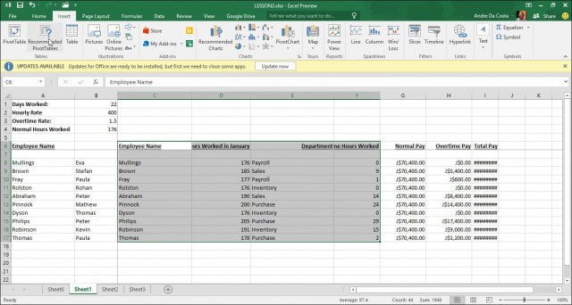
Introduced in Excel 2013, a Recommended Pivot Table is a predesigned summary of your data that Excel recommends for you. You might not get the information you need depending on your data set, but it can be handy for quick analysis. To create one, highlight the data source (the range of cells in the workbook that contains the data you want to analyze.) Then select the Insert tab and then Recommended PivotTables.

When the Choose Data Source dialog appears, click OK.

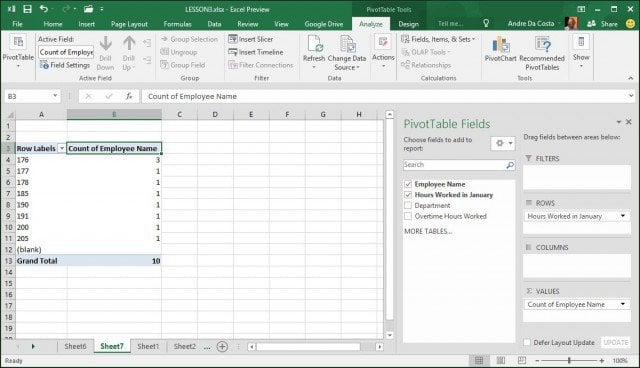
A gallery of recommended PivotTable styles will appear that provides suggestions for how you might want to analyze the selected data. In the following example, I’ll go with the Count of Employee Name by Hours Worked in January. Yours will vary depending on the type of data you are sorting. Click OK.

As you can see in the table below, I can get an idea of how many persons worked a certain amount of hours in January. A scenario like this would be great to see who might be working the hardest, working overtime, and from which department within a company.

Dig in

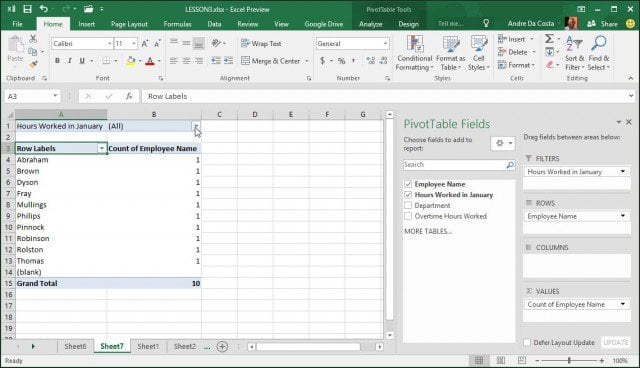
To make it more interesting, let’s dig in further and find out which employee is working the most. As you can see, the Pivot Table task pane appears on the right, displaying additional tools I can use to sort and filter. For the following example, I will add the Hours Worked in January to the Filters area and add the employee name to the Row area. After doing that, you will notice a new field added to the sheet called Hours Worked in January.

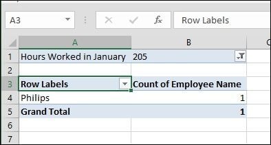
When I click in the filter box, I can see the lowest and the highest. Let’s select the highest, which is 205, click OK. So an employee by the name of Philip worked the most hours in January. It doesn’t get any easier than that.

Create a PivotTable from Scratch

If you want more control over how your pivot table is designed, you can do it yourself using the standard Pivot Table tool. Again, select the data source or the range where the data is stored in the workbook and select Insert > PivotTable.

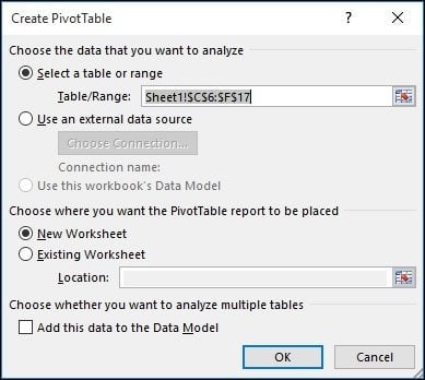
A Create PivotTable dialog appears with multiple options. Since I’m working with the data source from within the worksheet itself, I’ll leave the default. You can choose to add the Pivot Table to an existing worksheet or a new one. In this case, I’ll insert it into a new sheet.

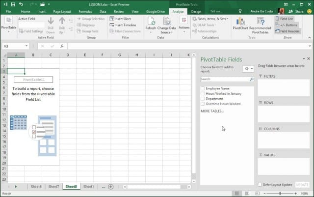
You will notice a new sheet appears with suggestions about what you can do. In this particular scenario, I want to know how many hours are worked by employees in Sales. To do that, I use Department to Filter down the list and add the other Tables to the Rows, such as the Employee Name and the number of hours worked.

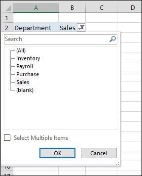
Click on the Department filter, then click Sales, and then OK.

Immediately, I can see who worked the most. I added an extra field for overtime to further analyze the information provided.

You should now have a good idea of how powerful Pivot Tables are. And how they save time by finding the exact information you need with little effort. For a small amount of data, this might be overkill. But for larger, more complex datasets, it makes your job a whole lot easier.